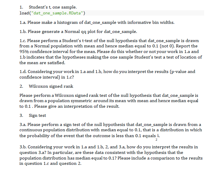
1. Student's t, one sample.

load("dat_one_sample. RData")

1.a. Please make a histogram of dat_one_sample with informative bin widths.

1.b. Please generate a Normal qq plot for dat_one_sample.

1.c. Please perform a Student's t-test of the null hypothesis that dat_one_sample is drawn

from a Normal population with mean and hence median equal to 0.1 (not 0). Report the

95% confidence interval for the mean. Please do this whether or not your work in 1.a and

1.b indicates that the hypotheses making the one sample Student's test a test of location of

the mean are satisfied.

1.d. Considering your work in 1.a and 1.b, how do you interpret the results (p-value and

confidence interval) in 1.c?

2. Wilcoxon signed rank

Please perform a Wilcoxon signed rank test of the null hypothesis that dat_one_sample is

drawn from a population symmetric around its mean with mean and hence median equal

to 0.1. Please give an interpretation of the result.

3. Sign test

3.a. Please perform a sign test of the null hypothesis that dat_one_sample is drawn from a

continuous population distribution with median equal to 0.1, that is a distribution in which

the probability of the event that the outcome is less than 0.1 equals ¹

2

3.b. Considering your work in 1.a and 1.b, 2, and 3.a, how do you interpret the results in

question 3.a? In particular, are these data consistent with the hypothesis that the

population distribution has median equal to 0.1? Please include a comparison to the results

in question 1.c and question 2./n4.

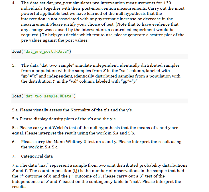
The data set dat_pre_post simulates pre-intervention measurements for 130

individuals together with their post-intervention measurements. Carry out the most

powerful applicable test we have learned of the null hypothesis that the

intervention is not associated with any systematic increase or decrease in the

measurement. Please justify your choice of test. (Note that to have evidence that

any change was caused by the intervention, a controlled experiment would be

required.) To help you decide which test to use, please generate a scatter plot of the

pre values against the post values.

load("dat_pre_post.RData")

5. The data "dat_two_sample" simulate independent, identically distributed samples

from a population with the samples from X in the "val" column, labeled with

"gp"="x" and independent, identically distributed samples from a population with

the distribution y in the "val" column, labeled with "gp"="y"

load("dat_two_sample. RData")

5.a. Please visually assess the Normality of the x's and the y's.

5.b. Please display density plots of the x's and the y's.

5.c. Please carry out Welch's test of the null hypothesis that the means of x and y are

equal. Please interpret the result using the work in 5.a and 5.b.

6. Please carry the Mann Whitney U test on x and y. Please interpret the result using

the work in 5.a-5.c.

7. Categorical data

7.a. The data "mat" represent a sample from two joint distributed probability distributions

X and Y. The count in position (ij) is the number of observations in the sample that had

the ith outcome of X and the jth outcome of Y. Please carry out a 3² test of the

independence of X and Y based on the contingency table in "mat". Please interpret the

results./nindependence of X and Y based on the contingency table in "mat". Please interpret the

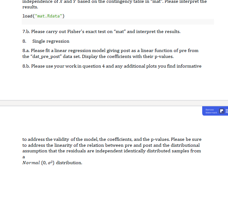
results.

load("mat.Rdata")

7.b. Please carry out Fisher's exact test on "mat" and interpret the results.

8. Single regression

8.a. Please fit a linear regression model giving post as a linear function of pre from

the "dat_pre_post" data set. Display the coefficients with their p-values.

8.b. Please use your work in question 4 and any additional plots you find informative

to address the validity of the model, the coefficients, and the p-values. Please be sure

to address the linearity of the relation between pre and post and the distributional

assumption that the residuals are independent identically distributed samples from

a

Normal (0, σ²) distribution.

Remove

Watermark

W

PC