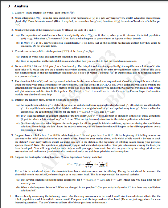
3 Analysis

1. Classify (1) and interpret (in words) each term of f(y).

2. When interpreting H(y), consider these questions: what happens to H(y) as y gets very large or very small? What does this represent

physically? Does this make sense? (Hint: It may help to remember that y' and, therefore, H(y) has units of hundreds of tribbles per

day.)

3. What are the units of the parameters a and b? (Recall the units of y and t)

4.

(a) Use separation of variables to solve (1) analytically when H(y) = 0, that is, when p = 0. Assume the initial population

y(0) = 30. What does a/b represent? (Hint: look at what happens to your solution as t grows without bound)

(b) If H (y) #0 in (1), can we still solve it analytically? If so, how? Set up the integrals needed and explain how they could be

evaluated. Do not evaluate them.

5. Consider an ordinary differential equation (ODE) of the form y = f(y).

(a) Define in words what an equilibrium solution to the equation is.

(b) Give an equivalent mathematical definition and explain how you use this to find the equilibrium solutions.

6. For b=0.005, 0.05, and 0.10, plot f as a function of y. Use this plot to determine (graphically) the equilibrium solutions of (1) for

each value of b. Make sure you use a suitable scale when plotting, so that you do not miss any equilibrium values. You can also use a

root finding routine to find the equilibrium solutions (e.g. fzero in Matlab). Plotting f(y) in Desmos may also be beneficial (enter b

as a parameter/slider).

7. Plot direction fields of (1) and overlay several solutions for the same values of b as in question 6. Consider the equilibrium solutions

when choosing your initial conditions for your solutions. You can do this in MATLAB (quiver command will aid in creating the

direction fields; you can code up Euler's method or use ode 45 to find solutions) or you can use the Geogebra script located here which

will plot solutions and direction fields together. The files dirfield.m and basic.ode45.m the Canvas Project Information

module may also be of some help.

8. Interpret the function plots, direction fields and solutions:

(a) An equilibrium solution y' is stable if, for a set of initial conditions in a neighborhood around y", all solutions are attracted to

y". An equilibrium is unstable if all initial conditions in a neighborhood of y" are repelled away from y. Make a table that

classifies all the equilibrium solutions for the plots b=0.005, b=0.05, and b=0.10.

(b) If y' is an equilibrium or constant solution of the first order ODE y = f(y), its basin of attraction is the set of initial conditions

(t.go) for which solutions tend to y" as too. What are the basins of attraction for the stable equilibrium solutions?

(c) Qualitatively describe what happens for each graph for all the possible initial conditions, again considering the equilibrium

solutions. Even though we don't know the analytic solution, can we determine what will happen to the tribble population over a

long period of time?

9. Suppose brown tribbles have b = 0.005, white have b = 0.05, and grey have b=0.10. At the beginning of tribbling season, we

can ensure the initial population to be at a certain value. Based on your results above, with which tribble would it be best to stock

the station? How many tribbles should we make sure are in the station at the beginning of tribbling season (using your previous

species choice)? Note: this question is intentionally vague and somewhat open-ended. Your job is to answer it using the tools you

have developed. You will be graded not only on how well you apply these tools, but also on your clarity in stating priorities and

assumptions and realizations (mathematically, computationally, etc.) of those priorities and assumptions.

10. Suppose the hunting/harvesting function, H, now depends on t and y, such that

py

H = H(t,y) = sin (5)

If t = 0 is the middle of winter, the sinusoidal term has a minimum so no one is tribbling. During the middle of the summer, the

sinusoidal term is maximized, so harvesting is at its maximum level. This is a simple model for seasonal variation.

(a) Plot several solutions (different initial conditions) for b=0.005, b = 0.05, and b = 0.10. Make sure you have time run for

several years.

(b) What is the long-term behavior? What has changed in the problem? Can you analytically solve it? Are there any equilibrium

solutions left?

11. Discuss briefly concerning the following issues. Are there any weaknesses in the model used? Are there additional effects that the

tribble population model should take into account? Can your model be improved and if so, how? (These are just suggestions for some

interesting questions. You don't have to address all of these questions in the report.)