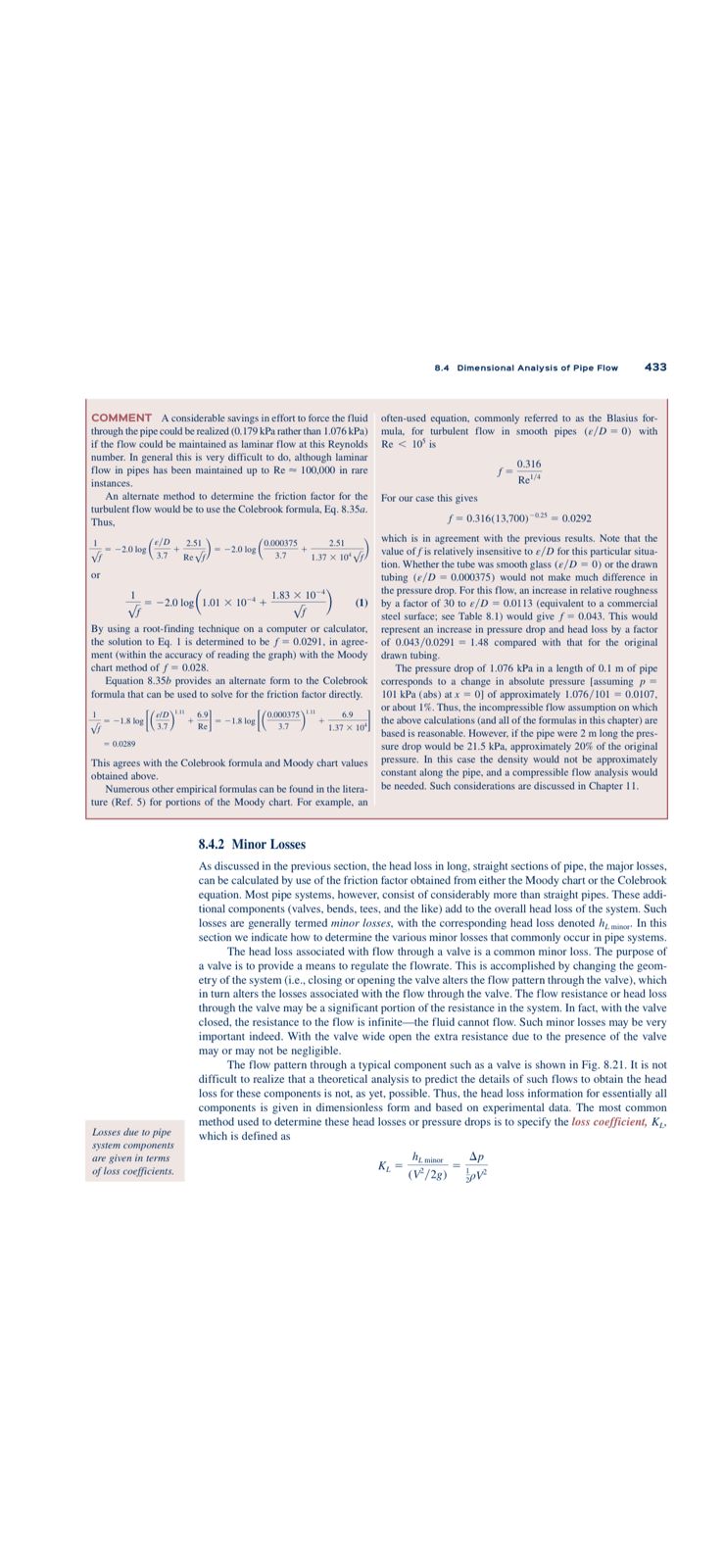
COMMENT A considerable savings in effort to force the fluid
through the pipe could be realized (0.179 kPa rather than 1.076 kPa)
if the flow could be maintained as laminar flow at this Reynolds
number. In general this is very difficult to do, although laminar
flow in pipes has been maintained up to Re 100,000 in rare
instances.
An alternate method to determine the friction factor for the For our case this gives
turbulent flow would be to use the Colebrook formula, Eq. 8.35a.
Thus,
1
VI
or
e/D
2.51
8 (37 +265/3) = -20 10g (030775
log
Rev
-2.0 log
-2.0 log 1.01 X 10+
0 log (1.0)
2.51
1.37 x 10 √f
1.83 x 10⁻⁴
By using a root-finding technique on a computer or calculator,
the solution to Eq. 1 is determined to be f = 0.0291, in agree-
ment (within the accuracy of reading the graph) with the Moody
chart method of f= 0.028.
Equation 8.35b provides an alternate form to the Colebrook
formula that can be used to solve for the friction factor directly.
Losses due to pipe
system components
are given in terms.
of loss coefficients.
-1.8 log (117)+--1.8 log[(0000375) +
-0.0289
This agrees with the Colebrook formula and Moody chart values
obtained above.
f-0.316(13,700)-25= 0.0292
which is in agreement with the previous results. Note that the
value of fis relatively insensitive to e/D for this particular situa-
tion. Whether the tube was smooth glass (e/D= 0) or the drawn
tubing (e/D= 0.000375) would not make much difference in
the pressure drop. For this flow, an increase in relative roughness
by a factor of 30 to e/D= 0.0113 (equivalent to a commercial
steel surface; see Table 8.1) would give f= 0.043. This would
represent an increase in pressure drop and head loss by a factor
of 0.043/0.0291 1.48 compared with that for the original
drawn tubing.
(1)
6.9
1.37 x 10¹
Numerous other empirical formulas can be found in the litera-
ture (Ref. 5) for portions of the Moody chart. For example, an
8.4 Dimensional Analysis of Pipe Flow
often-used equation, commonly referred to as the Blasius for-
mula, for turbulent flow in smooth pipes (e/D=0) with
Re< 10' is
f-
K₁ =
433
0.316
Rel/4
The pressure drop of 1.076 kPa in a length of 0.1 m of pipe
corresponds to a change in absolute pressure [assuming p=
101 kPa (abs) at x = 0] of approximately 1.076/101= 0.0107,
or about 1%. Thus, the incompressible flow assumption on which
the above calculations (and all of the formulas in this chapter) are
based is reasonable. However, if the pipe were 2 m long the pres-
sure drop would be 21.5 kPa, approximately 20% of the original
pressure. In this case the density would not be approximately
constant along the pipe, and a compressible flow analysis would
be needed. Such considerations are discussed in Chapter 11.
8.4.2 Minor Losses
As discussed in the previous section, the head loss in long, straight sections of pipe, the major losses,
can be calculated by use of the friction factor obtained from either the Moody chart or the Colebrook
equation. Most pipe systems, however, consist of considerably more than straight pipes. These addi-
tional components (valves, bends, tees, and the like) add to the overall head loss of the system. Such
losses are generally termed minor losses, with the corresponding head loss denoted h minor In this
section we indicate how to determine the various minor losses that commonly occur in pipe systems.
The head loss associated with flow through a valve is a common minor loss. The purpose of
a valve is to provide a means to regulate the flowrate. This is accomplished by changing the geom-
etry of the system (i.e., closing or opening the valve alters the flow pattern through the valve), which
in turn alters the losses associated with the flow through the valve. The flow resistance or head loss
through the valve may be a significant portion of the resistance in the system. In fact, with the valve
closed, the resistance to the flow is infinite-the fluid cannot flow. Such minor losses may be very
important indeed. With the valve wide open the extra resistance due to the presence of the valve
may or may not be negligible.
hy minor
(V²/28)
The flow pattern through a typical component such as a valve is shown in Fig. 8.21. It is not.
difficult to realize that a theoretical analysis to predict the details of such flows to obtain the head
loss for these components is not, as yet, possible. Thus, the head loss information for essentially all
components is given in dimensionless form and based on experimental data. The most common
method used to determine these head losses or pressure drops is to specify the loss coefficient, K₁,
which is defined as
Ap
p