GO! with Microsoft® Office 2019 Scripted Lecture for GO! with Microsoft Office 2019 Excel Chapter 1 Project 1B To the instructor: The notes below are provided for you to demonstrate to your students the skills they will practice when they create Project 1B. Although the skills and approach are identical to Project 1B, the content is different from the actual text. As necessary, refer to the steps in the text and Excel_1B_script_solution as your guide as you demonstrate. You may find it easier if you place the solution file on the desktop. Point out that the workbook should be saved after each activity. Activity Name Objective 7: Check Spelling in a Worksheet 1.18 Check Spelling in a Worksheet Demonstration Notes Start Excel and display a new blank workbook. • Save the workbook as Excel_1B_script_solution In cell A1: Type Western Mountains Warehouse and press Enter. Type Exercise Equipment Inventory In cell B3: Type Quantity and press Tab. Type Average Cost and press Tab. Type Retail Price and press Tab. Type Total Retail Value and press Tab. Type Percent of Total Retail Value and press Enter. In cell A4, type Traedmill with the text spelled incorrectly and then press Enter. In the range A5:A8 type the following row titles: Rowers Elliptical Trainers Exercise Bike Total Retail Value for All Products Adjust the width of column A to 220 pixels. Merge and Center the text in the range A1:F1 and then apply the Title style. Merge and Center the text in the range A2:F2 and then apply the Heading 1 style. Check Spelling for entire worksheet, making necessary corrections. Objective 8: Enter Data by Range 1.19 Entering Data by Range Select the range B4:D7. Pressing Enter after each entry with B4 as the active cell, type the following: 533 612 833 988 With cell C4 active, continue to type the following values, pressing Enter after each: Average Cost Retail Price 620 735 3350 4380 385 550 270 350/nObjective 9: Construct Formulas for Mathematical Operations 1.20 Using Arithmetic Operators 1.21 Tool 1.22 Using the Quick Analysis Copying Formulas Containing Absolute Cell References |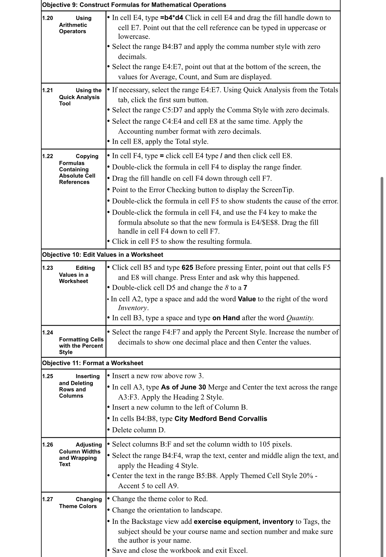In cell E4, type =b4*d4 Click in cell E4 and drag the fill handle down to cell E7. Point out that the cell reference can be typed in uppercase or lowercase. • Select the range B4:B7 and apply the comma number style with zero decimals. • Select the range E4:E7, point out that at the bottom of the screen, the values for Average, Count, and Sum are displayed. If necessary, select the range E4:E7. Using Quick Analysis from the Totals tab, click the first sum button. • Select the range C5:D7 and apply the Comma Style with zero decimals. Select the range C4:E4 and cell E8 at the same time. Apply the Accounting number format with zero decimals. In cell E8, apply the Total style. In cell F4, type = click cell E4 type / and then click cell E8. Double-click the formula in cell F4 to display the range finder. Drag the fill handle on cell F4 down through cell F7. Point to the Error Checking button to display the ScreenTip. Double-click the formula in cell F5 to show students the cause of the error. • Double-click the formula in cell F4, and use the F4 key to make the formula absolute so that the new formula is E4/$E$8. Drag the fill handle in cell F4 down to cell F7. Click in cell F5 to show the resulting formula. Objective 10: Edit Values in a Worksheet 1.23 1.24 Editing Values in a Worksheet Formatting Cells with the Percent Style • Click cell B5 and type 625 Before pressing Enter, point out that cells F5 and E8 will change. Press Enter and ask why this happened. • Double-click cell D5 and change the 8 to a 7 In cell A2, type a space and add the word Value to the right of the word Inventory. In cell B3, type a space and type on Hand after the word Quantity. Select the range F4:F7 and apply the Percent Style. Increase the number of decimals to show one decimal place and then Center the values. Objective 11: Format a Worksheet Inserting 1.25 and Deleting 1.26 1.27 Rows and Columns Adjusting Column Widths and Wrapping Text Changing Theme Colors Insert a new row above row 3. In cell A3, type As of June 30 Merge and Center the text across the range A3:F3. Apply the Heading 2 Style. Insert a new column to the left of Column B. In cells B4:B8, type City Medford Bend Corvallis •Delete column D. Select columns B:F and set the column width to 105 pixels. Select the range B4:F4, wrap the text, center and middle align the text, and apply the Heading 4 Style. Center the text in the range B5:B8. Apply Themed Cell Style 20% - Accent 5 to cell A9. Change the theme color to Red. • Change the orientation to landscape. In the Backstage view add exercise equipment, inventory to Tags, the subject should be your course name and section number and make sure the author is your name. Save and close the workbook and exit Excel.

Fig: 1

Fig: 2