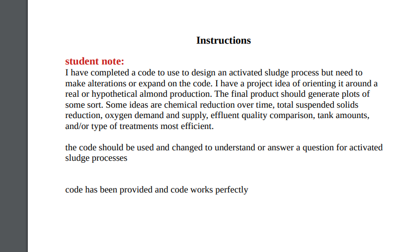
Instructions student note: I have completed a code to use to design an activated sludge process but need to make alterations or expand on the code. I have a project idea

of orienting it around a real or hypothetical almond production. The final product should generate plots of some sort. Some ideas are chemical reduction over time, total suspended solids reduction, oxygen demand and supply, effluent quality comparison, tank amounts, and/or type of treatments most efficient. the code should be used and changed to understand or answer a question for activated sludge processes code has been provided and code works perfectly/n Assignment Perform a preliminary design of an activated sludge process for a location that you select. The entire design process should be driven by a specific reason and/or objective. Clearly articulate what the reason and/or objective is/are, and perform a critical analysis of design options you considered in reaching your final design. Specify the size of the tanks, the recycle ratio, the mean cell residence time, the flow distribution, any process modifications anticipated in the future, any process modifications anticipated over the course of a year, and all relevant information pertaining to the aeration system. Clearly state all assumptions. The final deliverable of this homework assignment is an engineering report. The report should include the following sections: Introduction, Methods, Results and Discussion, Conclusions, and References. Please provide your source code in an appendix of your report. Your grade for this assignment will be based in part on how well your design approach reflects your reasons/objectives for design, critical analysis of design options, reasonableness of your design, and the quality of your writing. The design of the activated sludge process will have to be performed in Python (or a programing language of your choice). I have provided a set of tasks below to help guide you through the process of developing Python code. Task 1: Get familiar with Python This goal of this task is to get a working installation of Python on your computer and to get you familiar with the programming language. When you become proficient with Python you will realize just how much more you can do with it compared to Excel. Follow the instructions for installing Anaconda (a distribution of Python with many wonderful packages conveniently installed) found here (https://docs.anaconda.com/anaconda/install/index.html). You will also need to have access to a text editor or IDE that facilitates writing code. I use VS Code (https://code.visualstudio.com/download). Feel free to use another option if you'd like. Spyder comes with Anaconda and is also an acceptable alternative. You can run python from the command line, as shown in the video linked below, or you can create a text file and then run that text file in a command window. Your Python text files should have a .py extension, not a .txt extension. To run the file in a command prompt, type “python filename.py”, assuming your command prompt has navigated to the same folder as the .py file is located in. Otherwise, you can use “python C:\ full \ of \ file \ filename.py" from any command prompt. This video (https://www.youtube.com/watch?v=I2wURDqiXdM) explains the key concepts that you will need (ignore the parts about creating classes). Watch it and try out the commands for yourself. Also watch this video (https://www.youtube.com/watch?v=xECXZ3tyONo) for information on the package numpy, which is an extremely useful package. Stackoverflow is a great resource that you should take advantage of. Someone has more than likely already answered your question there. Once you have Python and an Editor installed on your computer,, do the following to start getting familiar with Python: 1. Print "hello world". 2. Create a list with the elements "red", "green", and "orange". 3. Create a dictionary with at least three keys. 4. Import the package numpy as np and use the exponential function to calculate e³. 5. Create a numpy array with values ranging from 0 to 10 (including 10). 6. Create a function that accepts an array, applies the function y(x) = −(1.2 − 4.3 * x) * sin(23 *x) to it, and returns the transformed array. 7. Import matplotlib as plt and use it to make a plot of the previously defined function from x = 0 to 10 (including 10). Include grid lines. Task 2 1. Create a Python file called SystemDefinition_AS.py. In this file create a function called SimulEQ(t,x,Q,V,Rates, Influent, MCRT,phi,rho). The arguments to this function have the following definitions: • • • • • • • Influent: A List of the influent concentrations of the So, Xvo, and Xdo. x: A List containing the initial guesses of all the unknowns. The unknowns are S1, S2, S3, S4, Xv1, Xv2, Xv3, Xv4, Xd1, Xd2, Xd3, Xd4. There is a total of 12 unknowns. Q: A scalar value representing the flow rate into the wastewater treatment plant. V: A List containing the scalar values of the volumes of each of the 4 tanks (V1, V2, V3, and V4). t: numeric value of the time step for the explicit finite difference method (you will use this in a later task). MCRT: A scalar value of mean cell residence time. Rates: A List containing scalar values of the following parameters: um, Ks, Ymax, b, gamma, beta (aka, mg of oxygen equivalents/mg of cells), alpha (aka, recycle ratio), kd (aka, used in the expression for Yobs). • phi: A List of the fraction of feed to tank 1, tank 2, tank 3, and tank 4. • rho: A List of the fraction of recycle to tank 1, tank 2, tank 3, and tank 4. This function should return a np.array that contains the 12 differential equations. 2. In the file SystemDefinition_AS.py create a function called getInit(). There are no arguments to this function. This function should return a List that contains the initial guesses of the 12 unknowns. 3. In the file SystemDefinition_AS.py create a function called getInfl(). There are no arguments to this function. This function should return a List that contains the influent values of the So, Xvo, and Xdo. Task 3 Create a file called PlotSolution.py. In this file, insert the following code. This code will allow you to plot a panel of figures that show your results for each component in the influent, tank 1, tank 2, tank 3, and tank 4 as a bar chart of the steady state solution. import matplotlib.pyplot as plt def PlotSolution(Influent, Sol, w,RAS): inf = Influent fig,axs = plt.subplots(nrows=5,ncols=1,figsize = (17,8)) axs[0].bar([1,2,3,4,5], [inf[0],Sol.y[0][-1],Sol.y[1][-1],Sol.y[2][-1],Sol.y[3][-1]]) axs[0].set_xticks([1,2,3,4,5]) axs[0].set_xticklabels([",",",","]) axs[0].set_title('S (mg/L)') axs[1].bar([1,2,3,4,5], [inf[1],Sol.y[4][-1],Sol.y[5][-1],Sol.y[6][-1],Sol.y[7][-1]]) axs[1].set_xticks([1,2,3,4,5]) axs[1].set_xticklabels([",",",","]) axs[1].set_title('Xv (mg/L)') axs[2].bar([1,2,3,4,5], [inf[2],Sol.y[8][-1],Sol.y[9][-1],Sol.y[10][-1],Sol.y[11][-1]]) axs[2].set_xticks([1,2,3,4,5]) axs[2].set_xticklabels([",",",","]) axs[2].set_title('Xd (mg/L)') print([1,2], [RAS[0],RAS[1]]) axs[3].bar([1,2], [RAS[0],RAS[1]]) axs[3].set_xticks([1,2]) axs[3].set_xticklabels(['Xvr','Xdr']) axs[3].set_title('Xras (mg/L)') axs[4].bar([1], w) axs[4].set_xticks([1]) axs[4].set_xticklabels(['$\omega$']) axs[4].set_title('Fraction of Q Wasted') plt.tight_layout() plt.savefig('FIGURES\\ComponentsBarChart.png',dpi=300) plt.show() 3 Task 4 Create a Python file called AS_Configuration.py. In this file, write the following code starting on line 1: import numpy as np import pandas as pd from scipy.integrate import solve_ivp from matplotlib import pyplot as plt import sys from SystemDefinition_AS import getInfl, getInit, SimulEQ from PlotSolution import PlotSolution Now, perform the following steps. First, call getInit() and assign what this function returns to a variable called init. Second, call getInfl() and assign what this function returns to a variable called Influent. Next, assign values to the variables Q, V, rho, phi, and Rates. Now we are going to solve the system of equations you wrote in the file SystemDefinition_AO.py contained in the function SimulEQ(...). The equations you wrote represent a system of ordinary differential equations (ODEs). We are going to solve these equations as an initial value problem using a function in scipy.integrate. Here is the code to do this: Sol = solve_ivp(fun = lambda t,y: SimulEQ(t,y,Q,V,Rates, Influent,MCRT,phi,rho), t_span= [0,1000], y0= init, dense_output=False, method = 'RK45') Please spend some time understanding this function and the output. Next, assign the output to variables that represent each of the components. Here is an example of the code that you can replicate. t = Sol.t S1 = Sol.y[0] S2 = Sol.y[1] S3 = Sol.y[2] S4 = Sol.y[3] Next, print the results of the output from solve.ivp for each component as a function of time. Here is an example of code that you can replicate. 4 fig, ax = plt.subplots(figsize=(10,10)) ax.plot(t,S1,label='S1') ax.plot(t,S2,label='S2') ax.plot(t,S3,label='S3') ax.plot(t,S4,label='S4') ax.legend() ax.set_ylabel('Concentration') ax.set_xlabel('Time') plt.savefig('FIGURES\\S.png',dpi = 300) Next calculate the values of w, Xvr, and Xdr. This will require you to pull out the last value in the index of values generated for Xv1, Xd1, Xv2, Xd2, Xv3, Xd3, Xv4, Xd4 from solve_ivp. I am intentionally not telling you how to do this so you have to understand the output from solve_ivp. Once you do this, create a variable called RAS that contains a List of the values for Xvr and Xdr. Finally, create a set of bar charts of the steady state concentrations of each of the components by calling: PlotSolution(Influent, Sol,w, RAS) Based on this output, as well as the time series plots you made of each component in each tank, check your results to make sure they make sense, possibly compare your results with other students (if you do this, you will have to make sure to use the same input values like for influent, Q, MCRT, V, etc), and fix any problems in the code. Task 5 Your code is now complete and is ready to use to design your activated sludge process. Run the code in whatever manner is necessary to complete the design of your activated sludge process. 5